Getting Started

Installing PySALESetup

PySALESetup can be installed simply using pip.

~/$ pip install pysalesetup

and requires Python 3.11+ to operate.

How to use PySALESetup

PySALESetup is designed to facilitate mesoscale iSALE simulation setup, and make it easy to construct complex geometries.

All PySALESetup workflows follow a simple pattern.

Create your model geometries. Your “plan”.
1. This includes object properties like velocity, and material.
Create your mesh, including extension zones.
Apply your geometries to the mesh and “populate” it.
Save your mesh/create input files

1. Create Objects & Geometries

The first step is to create the geometries that represent your model. The central object in this step is the PySALEObject. All workflow revolves around it. In order to create a new object you must instantiate PySALEObject and then set the various properties it possesses in order to configure it to your liking. This step is like drawing out a blueprint of the model. You define in physical space the ideal dimensions of your model, before it is applied to your imperfect mesh. All distances are in metres in this library.

PySALEObject possesses several methods which make it easy to create complex shapes, however, providing a list of tuple coordinates is enough to create a simple polygon.

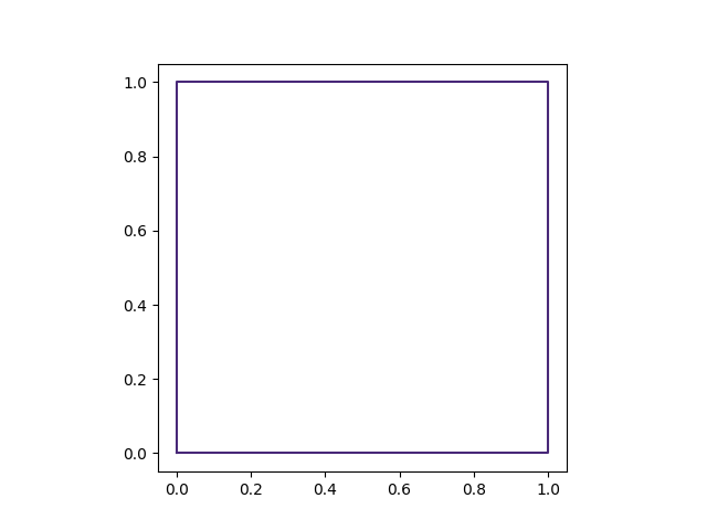
For example, we can create a 1m x 1m square like so:

from PySALESetup import PySALEObject
square = PySALEObject([(0, 0), (1, 0), (1, 1), (0, 1)])
fig, ax = square.plot()

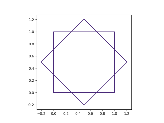
PySALEObject will also let you resize, rotate, and translate any objects you create after creation. Although you should note that these are not done in place. New objects are created each time.

from PySALESetup import PySALEObject
square = PySALEObject([(0, 0), (1, 0), (1, 1), (0, 1)])
diamond = square.rotate(45.)
fig, ax = square.plot()
diamond.plot(ax)

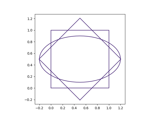
PySALEObject also includes several class methods that allow for the creation of common shapes that are not easy to define as a list of vertices. These are PySALEObject.generate_ellipse and PySALEObject.create_from_file. These methods create an elliptical object and an object based on a list of vertices in csv text file. PySALESetup contains its own grain library of text files with example grains (See GrainLibrary) which can be loaded in and used.

To create an ellipse we call the class method generate_ellipse and provide an origin coordinate as a list, followed by major axis, and minor axis and the amount of rotation. We can also specify an the origin about which the ellipse is rotated but by leaving it blank we default to the centre of the object.

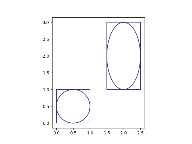
from PySALESetup import PySALEObject
square = PySALEObject([(0, 0), (1, 0), (1, 1), (0, 1)])
diamond = square.rotate(45.)
ellipse = PySALEObject.generate_ellipse([.5, .5], .7, .4, 0.)
fig, ax = square.plot()
diamond.plot(ax)
ellipse.plot(ax)

Note on circles in PySALESetup

PySALEObjects are always polygons. It is actually impossible in PySALESetup to create a perfect, circle. This is because PySALESetup will only create polygons. This is functionally irrelevant, however, because so many points are used that the result is indistinguishable from a circle in the imperfect meshes these objects are mapped to.

Object Children

PySALESetup was originally created to increase the flexibility of mesoscale mesh construction in iSALE. This included particle beds, and granular setups that got quite complex at times, with grains of different sizes, and shapes, in very specific arrangements. These capabilities are still present in this new version of PySALESetup and they revolve around the PySALEDomain object.

All PySALEObjects can have child objects associated with them. These are typically inside the parent’s bounds (although technically they don’t have to be). They _can_ be spawned from the parent and then manipulated as wanted, but normally you will want to create a “domain” instead. There is one, crucial, property of an object and its children that gives it an extraordinary amount of flexibility: translations/rotations/resizes will be applied to the parent and all its children recursively.

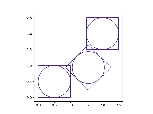
As such, you can do things like this:

from PySALESetup import PySALEObject

particle_bed = PySALEObject([(0, 0), (0, 1), (1, 1), (1, 0)])
ellipse = particle_bed.spawn_ellipse_in_shape([0.5, 0.5], .5, .5, 0)

new_bed1 = particle_bed.rotate(90, origin=(0.5, 2.))
new_bed2 = particle_bed.rotate(45, origin=(0.5, 2.))

f, a = particle_bed.plot()
new_bed1.plot(a)
new_bed2.plot(a)

or this

from PySALESetup import PySALEObject

particle_bed = PySALEObject([(0, 0), (0, 1), (1, 1), (1, 0)])
ellipse = particle_bed.spawn_ellipse_in_shape([0.5, 0.5], .5, .5, 0)
new_bed1 = particle_bed.rotate(90, origin=(0.5, 2.))
new_bed2 = new_bed1.resize(xfactor=1., yfactor=2.)

f, a = particle_bed.plot()
new_bed2.plot(a)

Domains

Creating child objects this way is all well and good for relatively simple setups. The object geometries could be complicated but realistically it will be fiddly to build many-object structures, like a full particle bed. This is where the PySALEDomain object comes in.

Domains are created from an existing PySALEObject. And essentially provide all the insertion methods you would need to build a particle bed(s). For example, it is relatively simple to create a bed of circles all of the same size.

from PySALESetup import PySALEObject, PySALEDomain

particle_bed = PySALEObject([(0, 0), (0, 1), (1, 1), (1, 0)])
grain = PySALEObject.generate_ellipse([0., 0.], .05, .05, 0)
domain = PySALEDomain(particle_bed)
achieved_area = domain.fill_with_random_grains_to_threshold(
    grain,
    threshold_fill_percent=50.
)
f, a = particle_bed.plot()
a.set_title(f'Filled to {achieved_area*100/particle_bed.area} %')

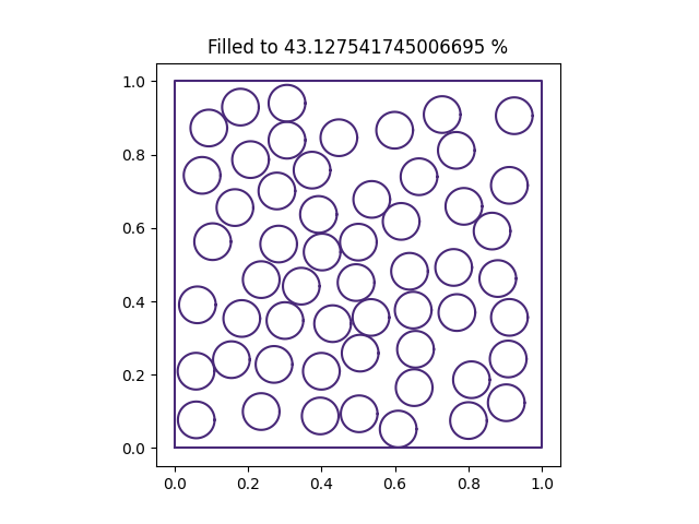
It is not always possible to achieve the specified threshold fill percent, but you can set the maximum number of retries with a grain before the code gives up as an optional argument. This defaults to 100.

But also, we can go further. We can supply a probability distribution for both the grain size and rotation, such that grains are drawn from these distributions when inserted. To do this we use the built-in PySALEDistribution classes. PySALESetup provides 4 distributions:

Uniform
Normal
Log Normal
Weibull 2-parameter

and one “custom” distribution object, which can be built using a CDF function and a random number function. So suppose we remade our bed in the previous example but with a uniform distribution in rotation and a normal distribution of grain sizes. Instead of a circle let’s use a rectangular base grain. Note: the size distribution is for the equivalent radius of the grain it is distributing. The equivalent radius is the radius of a circle with the same area as the grain in question.

from PySALESetup import PySALEObject, PySALEDomain, \
    PySALENormalDistribution, PySALEUniformDistribution

particle_bed = PySALEObject([(0, 0), (0, 1), (1, 1), (1, 0)])
grain = PySALEObject([(0, 0), (0, .05), (.05, .05), (.05, 0)])
domain = PySALEDomain(particle_bed)
achieved_area = domain.fill_with_random_grains_to_threshold(
    grain,
    threshold_fill_percent=50.,
    size_distribution=PySALENormalDistribution(.03, .003),
    rotation_distribution=PySALEUniformDistribution((0., 90.))
)
f, a = particle_bed.plot()
a.set_title(f'Filled to {achieved_area*100/particle_bed.area} %')

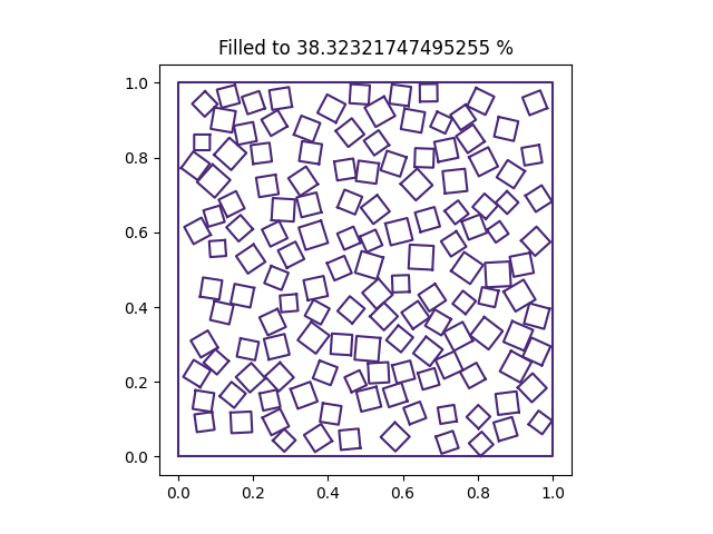
Grains generated like this will always be generated entirely within the parent object.

Set object properties

The final part of the first step is to set the properties of the objects. This boils down to: setting materials and velocities. This can be done directly on the objects, or it can be done through the domain, which leverages an optimise_materials method which will makes sure that the material numbers of all children in the domain are as far apart as they can be.

So to take our earlier example and add an impactor as well as materials and velocities we get this.

from PySALESetup import PySALEObject, PySALEDomain, \
    PySALENormalDistribution, PySALEUniformDistribution

particle_bed = PySALEObject([(0, 0), (0, 1), (1, 1), (1, 0)])
grain = PySALEObject([(0, 0), (0, .05), (.05, .05), (.05, 0)])
domain = PySALEDomain(particle_bed)
achieved_area = domain.fill_with_random_grains_to_threshold(
    grain,
    threshold_fill_percent=50.,
    size_distribution=PySALENormalDistribution(.03, .003),
    rotation_distribution=PySALEUniformDistribution((0., 90.))
)

impactor = PySALEObject([(0, 0), (0, 1),
                         (1, 1), (1, 0)]).translate(0.5, 1.5)
impactor.set_material(1)
impactor.set_velocity(0, -1000.)
particle_bed.set_material(2)
domain.optimise_materials([3, 4, 5, 6, 7, 8, 9])
f, a = particle_bed.plot()
impactor.plot(a)
a.set_title(f'Filled to {achieved_area*100} %')

You can see that the material numbers are reflected in the plots as well!

At this point we’re done with our drawing and ready to apply our simple model to a mesh.

2. Apply Your Geometries to a Mesh

The next few steps are significantly simpler than the first step. The geometries we’ve constructed in the previous sections are like templates. we can now apply those to a mesh. The PySALEMesh object is what we’ll use for this.

There are 2 ways to construct the mesh, and the choice depends on how you think about the model.

Give the number of cells and the cell size
Give the physical dimensions and the cell size

Both are valid approaches. For example to make a 100 x 100 mesh that is 1m x 1m we can either do

or

Both will produce the same result. Once we have a mesh instance all we need to do is make use of the method project_polygons_onto_mesh to apply whichever objects we wish to the mesh. As with the translate/resize/rotate methods, objects and their children are applied recursively.

With this in mind lets create a mesh for our example from the previous section.

from PySALESetup import PySALEObject, PySALEDomain, \
    PySALENormalDistribution, PySALEUniformDistribution, \
    PySALEMesh

particle_bed = PySALEObject([(0, 0), (0, 1), (1, 1), (1, 0)])
grain = PySALEObject([(0, 0), (0, .05), (.05, .05), (.05, 0)])
domain = PySALEDomain(particle_bed)
achieved_area = domain.fill_with_random_grains_to_threshold(
    grain,
    threshold_fill_percent=50.,
    size_distribution=PySALENormalDistribution(.03, .003),
    rotation_distribution=PySALEUniformDistribution((0., 90.))
)

impactor = PySALEObject([(0, 0), (0, 1),
                         (1, 1), (1, 0)]).translate(0.5, 1.5)
impactor.set_material(1)
impactor.set_velocity(0, -1000.)
particle_bed.set_as_void()
domain.optimise_materials([2, 3, 4, 5, 6, 7, 8, 9])

mesh = PySALEMesh.from_dimensions((1., 2.), 0.002)
mesh.project_polygons_onto_mesh([particle_bed])
mesh.project_polygons_onto_mesh([impactor])
f, a = mesh.plot_materials()

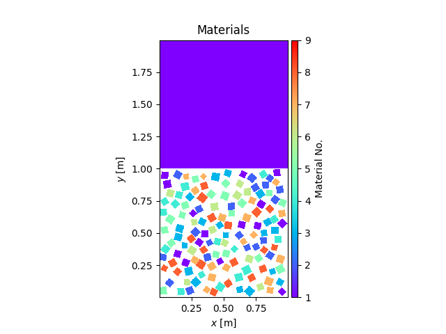
There is a plot_velocities method as well.

4. Create Input Files

The final step is to create input files. This is the simplest of all the steps. All we need to do is import the asteroid.inp and additional.inp creators and call one additional method on the mesh object save. save saves the mesh to a meso_m.iSALE file which can then be read by iSALE. You can optionally compress it using gzip as well.

The input file creation classes (AsteroidInput and AdditionalInput) are a little different but don’t require much additional effort. Mainly they require some additional inputs and eventually should be capable of creating the entire .inp files in their entirety. But for now, they have more limited abilities. But we do still need to supply a TimeStep object to the AsteroidInput class, which is just a named tuple.

Our final script looks like this:

from PySALESetup import PySALEObject, PySALEDomain, \
    PySALENormalDistribution, PySALEUniformDistribution, \
    PySALEMesh, AsteroidInput, AdditionalInput, TimeStep
import pathlib

particle_bed = PySALEObject([(0, 0), (0, 1), (1, 1), (1, 0)])
grain = PySALEObject([(0, 0), (0, .05), (.05, .05), (.05, 0)])
domain = PySALEDomain(particle_bed)
achieved_area = domain.fill_with_random_grains_to_threshold(
    grain,
    threshold_fill_percent=50.,
    size_distribution=PySALENormalDistribution(.03, .003),
    rotation_distribution=PySALEUniformDistribution((0., 90.))
)

impactor = PySALEObject([(0, 0), (0, 1),
                         (1, 1), (1, 0)]).translate(0.5, 1.5)
impactor.set_material(1)
impactor.set_velocity(0, -1000.)
particle_bed.set_as_void()
domain.optimise_materials([2, 3, 4, 5, 6, 7, 8, 9])

mesh = PySALEMesh.from_dimensions((1., 2.), 0.002)
mesh.project_polygons_onto_mesh([particle_bed])
mesh.project_polygons_onto_mesh([impactor])
mesh.save(pathlib.Path('./meso_m.iSALE'))

AsteroidInput('my_model',
              TimeStep(4.e-10, 1.e-8, 4.e-6, 1.e-7),
              mesh).write_to(pathlib.Path('./asteroid.inp'))
AdditionalInput(
    mesh,
    material_names={i: f'matter{i}' for i in range(1, 10)}
).write_to(pathlib.Path('./additional.inp'))

Running this in iSALE produces the following results.